Table of Contents
- Prerequisites
- Step 1 - Setting Up the Environment
- Step 2 - Basic Train-Test Split with Scikit-learn
- Step 3 - Reproducible Splits with Random Seeds
- Step 4 - Stratified Splits for Balanced Classes
- Step 5 - Train-Validation-Test Split
- Step 6 - Visualizing Splits
- Step 7 - Train-Test Splits with PyTorch
- Conclusion
When building a machine learning model, one of the first and most important steps is to evaluate its performance on data it has never seen before. This is where the concept of a train-test split comes in.
A train-test split is the process of dividing your dataset into two (or sometimes three) parts:
- Training set → used by the model to learn patterns.
- Testing set → used to evaluate the model’s performance on unseen data.
- (Optional) Validation set → used during training to fine-tune hyperparameters.
Without a proper split, your model might memorize the training data instead of learning general patterns, leading to overfitting. By splitting the dataset, you create a more realistic testing scenario that mirrors how your model will behave in the real world.
In this tutorial, you’ll learn how to perform train-test splits step by step on an Ubuntu 24.04 GPU server.
Prerequisites
- An Ubuntu 24.04 server with an NVIDIA GPU.
- A non-root user or a user with sudo privileges.
- NVIDIA drivers are installed on your server.
Step 1 – Setting Up the Environment
Before we dive into splitting datasets, we need to prepare our Ubuntu 24.04 GPU server with the right tools. This involves installing Python, creating a virtual environment, and setting up the required libraries for machine learning.
1. Install Python and other tools.
apt install -y python3 python3-venv python3-pip git2. Create and activate a virtual environment.
python3 -m venv ml-env
source ml-env/bin/activate
3. Update pip to the latest version.
pip install --upgrade pip4. Install required Python libraries.
pip install torch torchvision torchaudio --index-url https://download.pytorch.org/whl/cu121
pip install scikit-learn pandas matplotlib
5. Check if your GPU is available for PyTorch.
python3 -c "import torch; print(torch.cuda.is_available())"Output.
TrueIf it prints True, your setup is ready for GPU-powered experiments.
Step 2 – Basic Train-Test Split with Scikit-learn
The most common way to split data in machine learning is by using the train_test_split function from scikit-learn. Let’s start with a simple example using the Iris dataset, a small dataset of flower measurements often used in ML demos.
1. Create a script.
nano train_test_split_demo.pyAdd the following code.
#!/usr/bin/env python3
import pandas as pd
from sklearn.model_selection import train_test_split
from sklearn.datasets import load_iris

# Load dataset
iris = load_iris(as_frame=True)
X = iris.data
y = iris.target

# Perform split (80% training, 20% testing)
X_train, X_test, y_train, y_test = train_test_split(
    X, y, test_size=0.2, random_state=42
)

print("Training set size:", X_train.shape)
print("Testing set size:", X_test.shape)
2. Run the script.
python3 train_test_split_demo.pyOutput shows that out of 150 samples, 120 are used for training and 30 for testing.
Training set size: (120, 4)
Testing set size: (30, 4)
This basic split is often enough for quick experiments. However, in real-world scenarios, reproducibility and balanced splits are important, which we’ll cover next.
Step 3 – Reproducible Splits with Random Seeds
When you randomly split a dataset, the results can differ each time you run the script. This may lead to inconsistent results during experiments. To solve this, we use a random seed (via the random_state parameter) to make splits reproducible.
1. Create a new script.
nano reproducible_split.pyAdd the following code:
#!/usr/bin/env python3
from sklearn.model_selection import train_test_split
from sklearn.datasets import load_iris

iris = load_iris(as_frame=True)
X = iris.data
y = iris.target

# Fixed seed
X_train, X_test, y_train, y_test = train_test_split(
    X, y, test_size=0.3, random_state=123
)

print("Train size:", X_train.shape)
print("Test size:", X_test.shape)
2. Run the script.
python3 reproducible_split.pyOutput.
Train size: (105, 4)
Test size: (45, 4)
This is very useful when comparing models or sharing code with others because it guarantees consistent results.
Step 4 – Stratified Splits for Balanced Classes
Sometimes datasets have imbalanced classes (e.g., more samples of one category than others). If you randomly split such a dataset, the training and testing sets might not reflect the same class proportions, which can bias your model.
To avoid this, we use a stratified split. This ensures that each class appears in the train and test sets with the same proportion as in the full dataset.
1. Create the script.
nano stratified_split.pyAdd the following code:
#!/usr/bin/env python3
import pandas as pd
from sklearn.model_selection import train_test_split
from sklearn.datasets import load_iris

iris = load_iris(as_frame=True)
X = iris.data
y = iris.target

# Stratified split
X_train, X_test, y_train, y_test = train_test_split(
    X, y, test_size=0.3, stratify=y, random_state=42
)

print("Training class distribution:\n", y_train.value_counts(normalize=True))
print("Testing class distribution:\n", y_test.value_counts(normalize=True))
2. Run the script.
python3 stratified_split.pyOutput.
Training class distribution:
 target
1    0.333333
0    0.333333
2    0.333333
Name: proportion, dtype: float64
Testing class distribution:
 target
2    0.333333
1    0.333333
0    0.333333
Name: proportion, dtype: float64
In the Iris dataset, each of the three flower types makes up exactly 33.3% of the data, and you can see that both training and testing sets preserve this distribution.
Stratified splits are especially useful for classification problems with imbalanced datasets, such as fraud detection or medical diagnoses.
Step 5 – Train-Validation-Test Split
In many projects, using just a train-test split isn’t enough. You also need a validation set to tune hyperparameters, compare models, and avoid overfitting before touching the test data.
1. Create a validation script.
nano train_val_test_split.pyAdd the following code.
#!/usr/bin/env python3
from sklearn.model_selection import train_test_split
from sklearn.datasets import load_iris

iris = load_iris(as_frame=True)
X = iris.data
y = iris.target

# First: temp + test
X_temp, X_test, y_temp, y_test = train_test_split(
    X, y, test_size=0.2, random_state=42
)

# Second: train + validation
X_train, X_val, y_train, y_val = train_test_split(
    X_temp, y_temp, test_size=0.25, random_state=42
)  # 0.25 of 0.8 = 0.2 overall

print("Train:", X_train.shape)
print("Validation:", X_val.shape)
print("Test:", X_test.shape)
2. Run the script.
python3 train_val_test_split.pyOutput.
Train: (90, 4)
Validation: (30, 4)
Test: (30, 4)
Explanation
- First, we split 80% for train+validation and 20% for test.
- Then, we split that 80% again into 75% training and 25% validation, which results in:
- 60% training (90 samples)
- 20% validation (30 samples)
- 20% testing (30 samples)
This ensures that your model selection process never touches the test set, keeping it as a true “final exam” for your model.
Step 6 – Visualizing Splits
Numbers are helpful, but sometimes it’s easier to see how your data is divided. A quick visualization of class distributions in the train and test sets can confirm that the split worked as expected.
1. Create a script for visualization.
nano split_visualization.pyAdd the following code.
#!/usr/bin/env python3
import matplotlib.pyplot as plt
from sklearn.model_selection import train_test_split
from sklearn.datasets import load_iris
iris = load_iris(as_frame=True)
X = iris.data
y = iris.target
X_train, X_test, y_train, y_test = train_test_split(
X, y, test_size=0.3, stratify=y, random_state=42
)
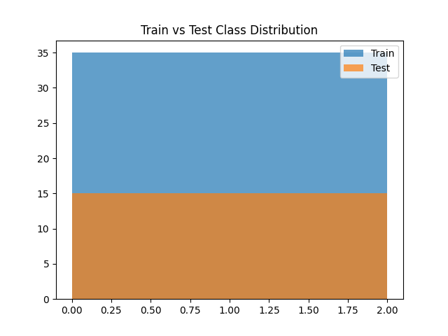
plt.hist(y_train, bins=len(set(y)), alpha=0.7, label="Train")
plt.hist(y_test, bins=len(set(y)), alpha=0.7, label="Test")
plt.legend()
plt.title("Train vs Test Class Distribution")
plt.savefig("split_distribution.png")
print("Visualization saved as split_distribution.png")2. Run the script.
python3 split_visualization.pyOutput.
Visualization saved as split_distribution.pngA file named split_distribution.png will be created in your project directory. Open it, and you’ll see a histogram comparing class counts in the training and test sets.
Step 7 – Train-Test Splits with PyTorch
So far, we’ve used scikit-learn for splitting datasets. But when working with deep learning in PyTorch, you’ll often load data into a TensorDataset and then split it using PyTorch utilities.
1. Create a script.
nano pytorch_split.pyAdd the following code.
#!/usr/bin/env python3
import torch
from torch.utils.data import random_split, TensorDataset
from sklearn.datasets import load_iris

# --- Suggested Change Start ---
# For reproducible splits, set the PyTorch random seed
torch.manual_seed(42)
# --- Suggested Change End ---

iris = load_iris(as_frame=True)
X = torch.tensor(iris.data.values, dtype=torch.float32)
y = torch.tensor(iris.target.values, dtype=torch.long)

dataset = TensorDataset(X, y)

# 80/20 split
train_size = int(0.8 * len(dataset))
test_size = len(dataset) - train_size
train_dataset, test_dataset = random_split(dataset, [train_size, test_size])

print("Train samples:", len(train_dataset))
print("Test samples:", len(test_dataset))
2. Run the script.
python3 pytorch_split.pyOutput.
Train samples: 120
Test samples: 30
Explanation
- TensorDataset(X, y) → bundles features and labels into a dataset PyTorch can work with.
- random_split → divides the dataset into train and test sets based on defined sizes.
- The split is compatible with PyTorch’s DataLoader, making it easy to feed batches into your model.
This approach is very common in deep learning workflows where datasets are stored as tensors rather than Pandas DataFrames.
Conclusion
In this guide, you explored the different ways to split datasets for machine learning on an Ubuntu 24.04 GPU server. You started with a simple train-test split using scikit-learn, then moved to reproducible splits with fixed seeds, balanced stratified splits, and extended the process to include a validation set. You also learned how to visualize splits for better understanding and performed splits directly in PyTorch for deep learning workflows.
* This post is for informational purposes only and does not constitute professional, legal, financial, or technical advice. Each situation is unique and may require guidance from a qualified professional.
Readers should conduct their own due diligence before making any decisions.