Table of Contents
- Prerequisites
- Step 1 - Install Dependencies
- Step 2 - Download NOAA Tornado Dataset
- Step 3 - Load and Inspect Data with Pandas
- Step 4 - Convert Tornado Events into GeoDataFrame
- Step 5 - Visualize Tornado Tracks
- Step 6 - Add U.S. State Boundaries and Hotspot Mapping
- Step 7 - GPU-Accelerated Analysis with cuDF
- Conclusion
Tornadoes are among the most destructive natural disasters in the United States, causing widespread damage to property, infrastructure, and human lives. Understanding where tornadoes occur and how they move is critical for risk assessment, emergency planning, and climate research.
In this tutorial, you’ll learn how to analyze tornado data using Python on an Ubuntu 24.04 GPU server. We’ll use NOAA’s (National Oceanic and Atmospheric Administration) Storm Events Dataset, which provides detailed records of tornado events, including their location, timing, and severity.
Prerequisites
- An Ubuntu 24.04 server with an NVIDIA GPU.
- A non-root user or a user with sudo privileges.
- NVIDIA drivers are installed on your server.
Step 1 – Install Dependencies
To start analyzing tornado data, you need the right tools installed on your Ubuntu 24.04 GPU server. We’ll set up Python, system libraries for geospatial processing, and Python packages for analysis and visualization.
1. GeoPandas and related libraries require GDAL and Fiona for handling spatial data. Install them along with Python tools.
apt install -y python3 python3-venv python3-pip git wget unzip gdal-bin libgdal-dev2. It’s a good practice to isolate dependencies in a virtual environment.
python3 -m venv tornado-env
source tornado-env/bin/activate
3. Next, upgrade pip and install the required Python libraries.
pip install --upgrade pip
pip install geopandas pandas matplotlib shapely pyproj fiona requests
These packages cover data analysis (pandas), geospatial processing (GeoPandas, Shapely, Fiona), and visualization (Matplotlib).
4. For larger datasets, GPU acceleration speeds up analysis. Install cudf-cu12 from NVIDIA’s PyPI index.
pip install cudf-cu12 --extra-index-url=https://pypi.nvidia.comThis gives you a pandas-like API that runs on the GPU for big-data tornado analysis.
Step 2 – Download NOAA Tornado Dataset
The National Oceanic and Atmospheric Administration (NOAA) maintains the Storm Events Database, which includes detailed records of tornadoes, floods, hurricanes, and other severe weather events across the United States. For this tutorial, we’ll focus on tornado events from the year 2010.
1. Create a directory for the dataset.
mkdir datasets && cd datasets2. Download the 2010 storm events CSV file.
wget https://www.ncei.noaa.gov/pub/data/swdi/stormevents/csvfiles/StormEvents_details-ftp_v1.0_d2010_c20250520.csv.gzThis file contains tornado records and other storm-related events for the year 2010.
3. Unzip the compressed file so it’s ready for analysis.
gunzip StormEvents_details-ftp_v1.0_d2010_c20250520.csv.gz4. Move back to the root directory to keep your workflow clean.
cd ..Step 3 – Load and Inspect Data with Pandas
Now that the dataset is downloaded and extracted, the first step is to load it into Python and explore its structure. We’ll use pandas, a powerful library for data analysis.
1. Create a script to load data.
nano load_data.pyAdd the following code.
#!/usr/bin/env python3
import pandas as pd

# Load tornado dataset
df = pd.read_csv("datasets/StormEvents_details-ftp_v1.0_d2010_c20250520.csv")

print("First five rows:")
print(df.head())
2. Run the script.
python3 load_data.pyOutput.
First five rows:
   BEGIN_YEARMONTH  BEGIN_DAY  BEGIN_TIME  ...                                  EPISODE_NARRATIVE                                    EVENT_NARRATIVE  DATA_SOURCE
0           201007          7        1251  ...  A strong ridge built into Southern New England...  Heat index values at the Nashua Boire Field (K...          CSV
1           201001         17        2300  ...  A coastal storm passing southern New England j...  Four to eight inches fell across eastern Hills...          CSV
2           201010          1         830  ...  Several waves of low pressure moved across Sou...  In Manchester, firefighters responded to about...          CSV
3           201007          6         951  ...  A strong ridge built into Southern New England...  Heat index values at the Manchester Airport (K...          CSV
4           201012         26        1700  ...  A strengthening winter storm passed southeast ...  Snowfall totals of 6 to 10 inches were observe...          CSV

[5 rows x 51 columns]
The NOAA Storm Events dataset contains over 50 columns. A few important ones for tornado analysis are:
- EVENT_TYPE – The type of storm (we’ll filter for Tornado).
- BEGIN_LAT / BEGIN_LON – The starting point of the tornado.
- END_LAT / END_LON – The ending point of the tornado.
- BEGIN_YEARMONTH, BEGIN_DAY, BEGIN_TIME – Date and time of the event.
- EVENT_NARRATIVE – A text description of what happened.
Step 4 – Convert Tornado Events into GeoDataFrame
Now that we’ve explored the dataset, the next step is to filter out tornado events and convert their coordinates into geospatial objects. This will allow us to map tornado tracks across the U.S. using GeoPandas.
1. Create a script for conversion.
nano convert_to_geodata.pyAdd the code below.
#!/usr/bin/env python3
import pandas as pd
import geopandas as gpd
from shapely.geometry import LineString

# Load dataset
df = pd.read_csv("datasets/StormEvents_details-ftp_v1.0_d2010_c20250520.csv")

# Filter only tornado events
df = df[df['EVENT_TYPE'] == 'Tornado']

print(f"Total tornado events: {len(df)}")

# Function to create LineString geometry (only if coords are valid)
def create_lines(row):
    if pd.notnull(row['BEGIN_LON']) and pd.notnull(row['BEGIN_LAT']) \
       and pd.notnull(row['END_LON']) and pd.notnull(row['END_LAT']):
        return LineString([(row['BEGIN_LON'], row['BEGIN_LAT']),
                           (row['END_LON'], row['END_LAT'])])
    return None

df['geometry'] = df.apply(create_lines, axis=1)

# Drop rows with invalid geometries
df = df.dropna(subset=['geometry'])

# Convert to GeoDataFrame
gdf = gpd.GeoDataFrame(df, geometry='geometry', crs="EPSG:4326")

print(gdf.head())
print(f"Valid tornado geometries: {len(gdf)}")
2. Run the script.
python3 convert_to_geodata.pyOutput.
Total tornado events: 1449
     BEGIN_YEARMONTH  BEGIN_DAY  BEGIN_TIME  ...                                    EVENT_NARRATIVE  DATA_SOURCE                                           geometry
75            201011         30          46  ...  An NWS Storm Survey found a weak EF0 tornado t...          CSV    LINESTRING (-92.1172 30.4366, -92.0965 30.4405)
304           201011         30        1945  ...  A tornado damage path was surveyed starting in...          CSV        LINESTRING (-82.605 34.829, -82.583 34.863)
617           201010         18        1643  ...  An EF-0 tornado, with winds estimated at 75 mp...          CSV  LINESTRING (-113.9737 35.2023, -113.9821 35.1859)
731           201011         29        1512  ...  Numerous trees were snapped near the intersect...          CSV     LINESTRING (-92.808 31.7947, -92.6528 31.9479)
732           201011         29        1618  ...  The tornado touched down in an inaccessible wo...          CSV    LINESTRING (-92.1872 32.2802, -92.1248 32.2864)

[5 rows x 52 columns]
Valid tornado geometries: 1449
You now have a GeoDataFrame of tornado paths ready for visualization. Next, we’ll plot these tornado tracks on a map using Matplotlib and GeoPandas.
Step 5 – Visualize Tornado Tracks
After converting tornado events into geospatial features, the next step is to plot tornado paths on a map. This gives us a clear visual representation of where tornadoes occurred and how they moved.
1. Create a script for plotting.
nano plot_tornado_paths.pyAdd the code below.
#!/usr/bin/env python3
import pandas as pd
import geopandas as gpd
from shapely.geometry import LineString
import matplotlib.pyplot as plt

# Load data
df = pd.read_csv("datasets/StormEvents_details-ftp_v1.0_d2010_c20250520.csv")

# Filter tornado events only
df = df[df['EVENT_TYPE'] == 'Tornado']

# Function to create LineString geometry
def create_lines(row):
    if pd.notnull(row['BEGIN_LON']) and pd.notnull(row['BEGIN_LAT']) \
       and pd.notnull(row['END_LON']) and pd.notnull(row['END_LAT']):
        return LineString([(row['BEGIN_LON'], row['BEGIN_LAT']),
                           (row['END_LON'], row['END_LAT'])])
    return None

df['geometry'] = df.apply(create_lines, axis=1)

# Drop invalid geometries
df = df.dropna(subset=['geometry'])

# Convert to GeoDataFrame
gdf = gpd.GeoDataFrame(df, geometry='geometry', crs="EPSG:4326")

print(f"Total tornado tracks to plot: {len(gdf)}")

# Plot tornado paths
fig, ax = plt.subplots(figsize=(12, 8))
gdf.plot(ax=ax, color="red", linewidth=1, alpha=0.7)

plt.title("Tornado Tracks - NOAA Storm Events (2010)", fontsize=16)
plt.xlabel("Longitude")
plt.ylabel("Latitude")

# Save figure
plt.savefig("tornado_tracks.png", dpi=300)
print("Map saved as tornado_tracks.png")
2. Run the script.
python3 plot_tornado_paths.pyOutput.
Total tornado tracks to plot: 1449
Map saved as tornado_tracks.png
This creates a file called tornado_tracks.png that shows tornado paths in red lines.
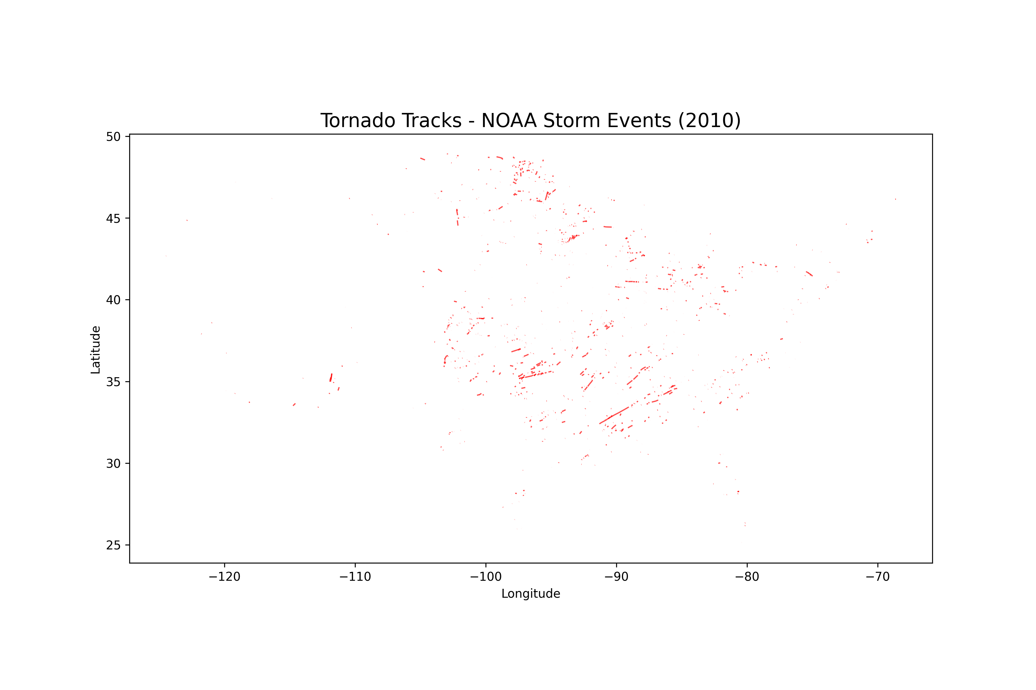
You now have a visual tornado map generated from NOAA’s dataset. Next, we’ll enhance this analysis by adding U.S. state boundaries and creating a hotspot (density) map.
Step 6 – Add U.S. State Boundaries and Hotspot Mapping
Plotting tornado paths gives us an overview, but to identify which states are most affected, we need to overlay tornado tracks with U.S. state boundaries. By performing a spatial join, we can count tornadoes per state and visualize hotspots.
1. Download the U.S. state shapefile.
wget https://www2.census.gov/geo/tiger/GENZ2018/shp/cb_2018_us_state_20m.zip
unzip cb_2018_us_state_20m.zip -d states
This creates a folder states/ containing the shapefile components.
2. Create a hotspot analysis script.
nano tornado_hotspots.pyAdd the following code.
#!/usr/bin/env python3
import pandas as pd
import geopandas as gpd
from shapely.geometry import LineString
import matplotlib.pyplot as plt

# Load tornado data
df = pd.read_csv("datasets/StormEvents_details-ftp_v1.0_d2010_c20250520.csv")


# Filter only tornado events
df = df[df['EVENT_TYPE'] == 'Tornado']

# Function to create LineString geometry
def create_lines(row):
    if pd.notnull(row['BEGIN_LON']) and pd.notnull(row['BEGIN_LAT']) \
       and pd.notnull(row['END_LON']) and pd.notnull(row['END_LAT']):
        return LineString([(row['BEGIN_LON'], row['BEGIN_LAT']),
                           (row['END_LON'], row['END_LAT'])])
    return None

df['geometry'] = df.apply(create_lines, axis=1)

# Drop invalid geometries
df = df.dropna(subset=['geometry'])

# Convert to GeoDataFrame
gdf = gpd.GeoDataFrame(df, geometry='geometry', crs="EPSG:4326")

print(f"Valid tornado tracks: {len(gdf)}")

# Load US state boundaries (NAD83)
states = gpd.read_file("states/cb_2018_us_state_20m.shp")

# Reproject states to match tornado CRS (WGS84)
states = states.to_crs(epsg=4326)

# Spatial join: tornadoes intersecting states
joined = gpd.sjoin(gdf, states, predicate="intersects")

# Count tornadoes per state
state_counts = joined.groupby("NAME")["EVENT_ID"].count().reset_index()

# Merge counts with state geometries
states = states.merge(state_counts, on="NAME", how="left")

# Plot tornado density
fig, ax = plt.subplots(figsize=(12, 8))
states.plot(column="EVENT_ID", cmap="Reds", legend=True, ax=ax, edgecolor="black")

plt.title("Tornado Density by State (2010)")
plt.savefig("tornado_density.png", dpi=300)
print("Hotspot map saved as tornado_density.png")
2. Run the script.
python3 tornado_hotspots.pyOutput.
Valid tornado tracks: 1449
Hotspot map saved as tornado_density.png
This creates a file tornado_density.png showing a choropleth map where states are shaded in red based on the number of tornadoes.
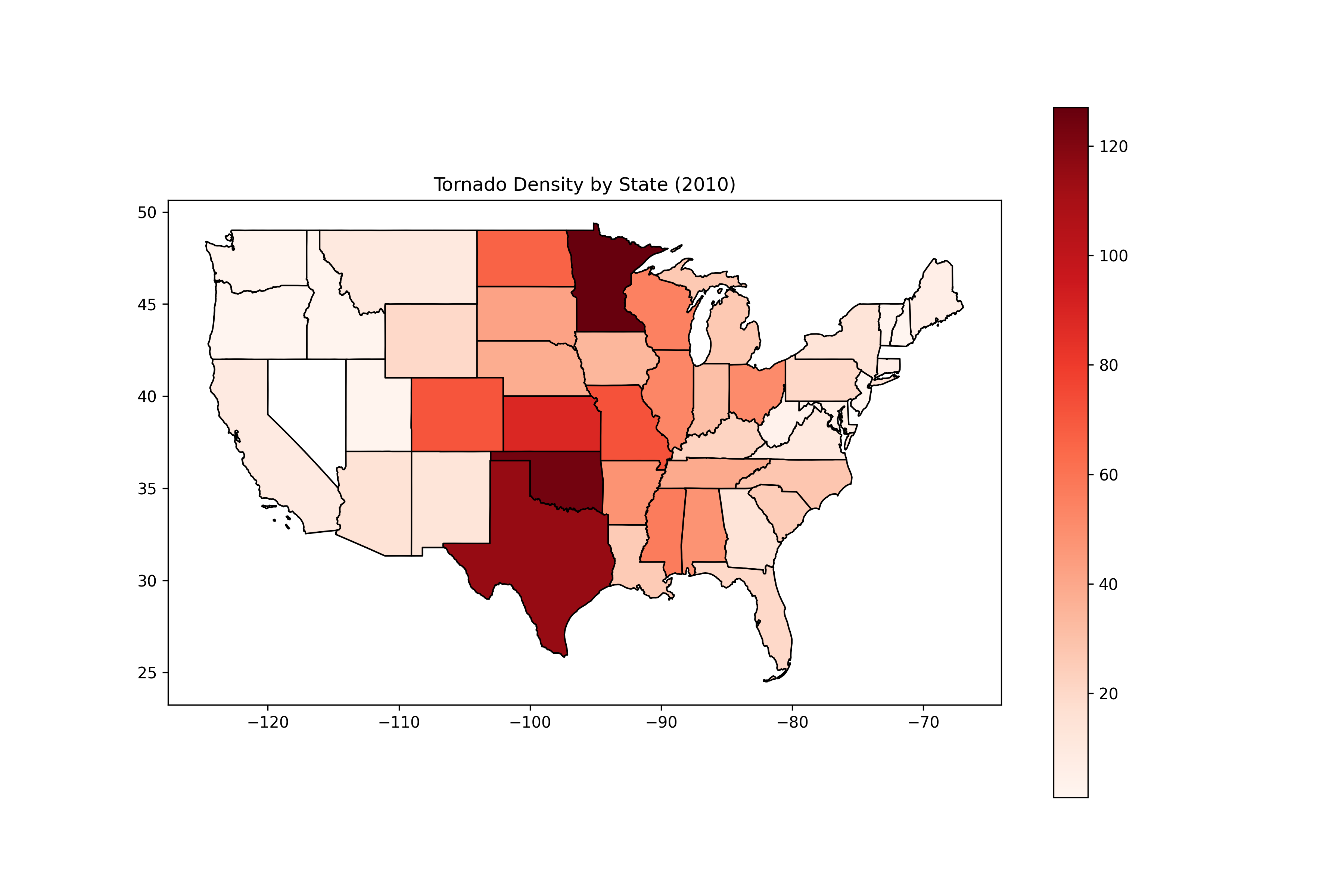
You now have a state-level tornado density map. Next, we’ll look at how to use GPU acceleration with cuDF to process this NOAA dataset much faster than pandas.
Step 7 – GPU-Accelerated Analysis with cuDF
When working with large NOAA storm event datasets (spanning decades), pandas on CPU can become slow. To speed things up, we can use cuDF, a RAPIDS library that mimics pandas but runs entirely on the GPU.
This lets us filter, aggregate, and explore millions of records with lightning-fast performance.
1. Create a script for GPU analysis.
nano gpu_analysis.pyAdd the following code.
#!/usr/bin/env python3
import cudf

df_gpu = cudf.read_csv("datasets/StormEvents_details-ftp_v1.0_d2010_c20250520.csv")
print(df_gpu.head())
2. Run the script.
python3 gpu_analysis.pyOutput.
   BEGIN_YEARMONTH  BEGIN_DAY  BEGIN_TIME  ...                                  EPISODE_NARRATIVE                                    EVENT_NARRATIVE  DATA_SOURCE
0           201007          7        1251  ...  A strong ridge built into Southern New England...  Heat index values at the Nashua Boire Field (K...          CSV
1           201001         17        2300  ...  A coastal storm passing southern New England j...  Four to eight inches fell across eastern Hills...          CSV
2           201010          1         830  ...  Several waves of low pressure moved across Sou...  In Manchester, firefighters responded to about...          CSV
3           201007          6         951  ...  A strong ridge built into Southern New England...  Heat index values at the Manchester Airport (K...          CSV
4           201012         26        1700  ...  A strengthening winter storm passed southeast ...  Snowfall totals of 6 to 10 inches were observe...          CSV

[5 rows x 51 columns]
With cuDF, we loaded NOAA data into GPU memory, filtered tornado events instantly, and grouped them by month at high speed. On multi-year datasets with millions of rows, cuDF can deliver 10x–50x faster performance than pandas, making it ideal for large-scale tornado analysis.
Conclusion
In this tutorial, you learned how to analyze tornado data from NOAA using Python, GeoPandas, and GPU acceleration with cuDF on Ubuntu 24.04. We loaded and inspected the dataset, converted tornado records into geospatial tracks, visualized their paths, mapped state-level hotspots, and leveraged GPU power for faster analysis.
This workflow shows how combining open datasets, geospatial libraries, and GPU acceleration can uncover meaningful insights into tornado patterns. You can extend this further by analyzing multiple years, comparing seasonal trends, or integrating population data to study risk impact.
* This post is for informational purposes only and does not constitute professional, legal, financial, or technical advice. Each situation is unique and may require guidance from a qualified professional.
Readers should conduct their own due diligence before making any decisions.