Anomalies are data points that deviate significantly from the majority of observations. Detecting them early can prevent fraud, identify cyberattacks, and flag unusual system behavior before it causes damage. This process is known as anomaly detection, and it plays a key role in fields such as banking (credit card fraud), cybersecurity (intrusion detection), and healthcare (disease pattern discovery).
Traditionally, anomaly detection methods run on CPUs, but with today’s growing datasets, CPU-based processing can become slow and inefficient. That’s where GPU acceleration comes in. Using NVIDIA’s RAPIDS cuML library, we can leverage the power of GPUs to speed up anomaly detection tasks dramatically. Instead of waiting minutes or hours, you can analyze massive datasets in seconds.
In this tutorial, you’ll learn how to perform anomaly detection on an Ubuntu 24.04 GPU server using Python and RAPIDS cuML.
Prerequisites
- An Ubuntu 24.04 server with an NVIDIA GPU.
- A non-root user or a user with sudo privileges.
- NVIDIA drivers are installed on your server.
Step 1 – Setting Up Python Environment
Before we start coding anomaly detection, we need to prepare a proper Python environment on our Ubuntu 24.04 GPU server.
1. Install Python tools.
apt install -y python3 python3-pip python3-venv python3-pip
2. Create a project directory.
mkdir anomaly-detection && cd anomaly-detection
3. Create and activate a virtual environment.
python3 -m venv .venv
source .venv/bin/activate
4. Upgrade pip and install dependencies.
pip install --upgrade pip
pip install numpy pandas matplotlib seaborn joblib scikit-learn
5. Finally, install cuML (RAPIDS library for GPU-accelerated ML).
pip install cuml-cu12 --extra-index-url=https://pypi.nvidia.com
Step 2 – Building a Synthetic Anomaly Detection Example
To understand how anomaly detection works with GPU acceleration, we’ll first create a synthetic dataset. This allows us to clearly visualize the difference between normal data points and anomalies before applying the method to a real-world dataset.
1. Create a Python script.
nano anomaly_detection_gpu.py
Add the following code.
# anomaly_detection_gpu.py
import numpy as np
import pandas as pd
import matplotlib.pyplot as plt
import seaborn as sns
from cuml.cluster import DBSCAN  # GPU-based DBSCAN
import joblib

# ------------------------------
# Step 1: Generate synthetic data
# ------------------------------
rng = np.random.RandomState(42)

# Normal points
X = 0.3 * rng.randn(200, 2)
X = np.r_[X + 2, X - 2]

# Outliers
outliers = rng.uniform(low=-6, high=6, size=(20, 2))
X = np.r_[X, outliers]

df = pd.DataFrame(X, columns=["feature1", "feature2"])

# ------------------------------
# Step 2: Train DBSCAN on GPU
# ------------------------------
# eps = neighborhood size, min_samples = density threshold
db = DBSCAN(eps=0.5, min_samples=5)
labels = db.fit_predict(df[["feature1", "feature2"]].values)

# Anomalies = label -1
df["anomaly"] = (labels == -1).astype(int)

print("Anomaly counts:")
print(df["anomaly"].value_counts())

# ------------------------------
# Step 3: Visualization
# ------------------------------
plt.figure(figsize=(8, 6))
sns.scatterplot(
    x="feature1", y="feature2",
    hue="anomaly", style="anomaly",
    palette={0: "blue", 1: "red"},
    data=df
)
plt.title("GPU Accelerated Anomaly Detection with cuML DBSCAN")
plt.savefig("anomaly_results.png")
plt.show()

# ------------------------------
# Step 4: Save model
# ------------------------------
# Save labels only (DBSCAN in cuML doesn’t support pickling yet)
joblib.dump(labels, "dbscan_labels.pkl")
print("Labels saved as dbscan_labels.pkl")
2. Run the script.
python3 anomaly_detection_gpu.py
You should see output similar to:
Anomaly counts:
anomaly
0    402
1     18
Name: count, dtype: int64
Labels saved as dbscan_labels.pkl
This indicates that the model identified 402 normal points and 18 anomalies.
3. The script saves a visualization as anomaly_results.png. Open it and you’ll see:
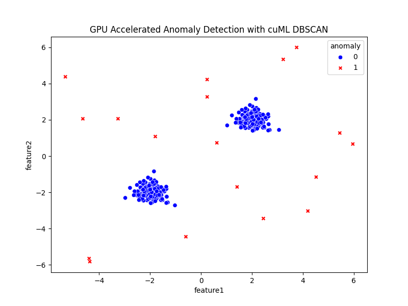
Blue points – Normal data
Red points – Detected anomalies
At this point, you have a working GPU-accelerated anomaly detection pipeline on synthetic data. Next, we’ll apply the same workflow to a real-world dataset: credit card fraud detection.
Step 3 – Applying to Real-World Dataset (Credit Card Fraud)
After testing on synthetic data, let’s scale up to a real-world dataset: the Credit Card Fraud Detection dataset. This dataset contains 284,807 transactions with 29 features, making it an excellent benchmark for anomaly detection.
1. Open a new Python file.
nano anomaly_creditcard_gpu.py
Add the following code.
import pandas as pd
from sklearn.datasets import fetch_openml
from cuml.cluster import DBSCAN
import joblib

# ------------------------------
# Step 1: Load Credit Card Fraud dataset
# ------------------------------
print("Downloading dataset...")
data = fetch_openml(name="creditcard", version=1, as_frame=True)
df = data.data

print("Dataset shape:", df.shape)

# ------------------------------
# Step 2: Train DBSCAN on GPU
# ------------------------------
db = DBSCAN(eps=3.0, min_samples=10)  # tune eps for better results
labels = db.fit_predict(df.values)

# Anomalies are labeled as -1
df["anomaly"] = (labels == -1).astype(int)

print("Anomaly counts:")
print(df["anomaly"].value_counts())

# ------------------------------
# Step 3: Save results
# ------------------------------
joblib.dump(labels, "creditcard_dbscan_labels.pkl")
df[["anomaly"]].to_csv("creditcard_anomalies.csv", index=False)

print("Labels saved as creditcard_dbscan_labels.pkl")
print("Anomaly flags saved to creditcard_anomalies.csv")
2. Run the script.
python3 anomaly_creditcard_gpu.py
You will see the following output.
Downloading dataset...
Dataset shape: (284807, 29)
Anomaly counts:
anomaly
0    218091
1     66716
Name: count, dtype: int64
Labels saved as creditcard_dbscan_labels.pkl
Anomaly flags saved to creditcard_anomalies.csv
Explanation:
- Dataset shape confirms the dataset size (284,807 rows × 29 features).
- Anomaly counts show how many transactions were flagged as suspicious (label 1) vs normal (label 0).
- creditcard_dbscan_labels.pkl – cluster labels for all transactions.
- creditcard_anomalies.csv – CSV file with anomaly flags (useful for further analysis in Excel, Pandas, or BI tools).
Conclusion
In this tutorial, you learned how to set up an Ubuntu 24.04 GPU server for anomaly detection with Python, build a synthetic dataset to test the workflow, and then scale the approach to a real-world credit card fraud dataset. Using RAPIDS cuML’s DBSCAN, we took advantage of GPU acceleration to handle clustering and anomaly detection much faster than traditional CPU-based methods.
* This post is for informational purposes only and does not constitute professional, legal, financial, or technical advice. Each situation is unique and may require guidance from a qualified professional.
Readers should conduct their own due diligence before making any decisions.