Autoencoders Using Keras on Ubuntu 24.04 GPU Server

Autoencoders are a special type of neural network designed to learn efficient representations of data. They’re commonly used for tasks like dimensionality reduction, image compression, and denoising. Instead of predicting labels, autoencoders aim to recreate their input at the output layer, forcing the network to learn the most important features in between.

In this hands-on tutorial, you’ll learn how to build several types of autoencoders using Keras with TensorFlow backend on an Ubuntu 24.04 GPU server.

Prerequisites

• An Ubuntu 24.04 server with an NVIDIA GPU.
• A non-root user or a user with sudo privileges.
• NVIDIA drivers are installed on your server.

Step 1: Set up Python Environment

Before diving into code, let’s prepare your Ubuntu 24.04 GPU server to run Keras-based autoencoders efficiently. This includes installing Python tools, setting up a virtual environment, and installing the required Python libraries.

1. Install Python tools and other dependencies.

apt install python3 python3-pip python3-venv git wget -y

2. Create and activate a virtual environment.

python3 -m venv autoencoder-env
source autoencoder-env/bin/activate

3. Now install TensorFlow, NumPy, and Matplotlib.

pip install --upgrade pip
pip install tensorflow matplotlib numpy

Explanation:

• tensorflow: Provides Keras API and GPU support
• matplotlib: Used to visualize image results
• numpy: Helps with array operations and data preprocessing

Step 2: Prepare MNIST Dataset

To train our autoencoders, we’ll use the MNIST dataset, a set of 70,000 handwritten digit images (28×28 pixels). This dataset is commonly used for testing image-based models because it’s lightweight and easy to visualize.

1. Download the MNIST dataset in .npz format from TensorFlow’s official hosting.

wget https://storage.googleapis.com/tensorflow/tf-keras-datasets/mnist.npz

This file contains:

• x_train: 60,000 training images
• y_train: labels for training data (we won’t use labels here)
• x_test: 10,000 test images
• y_test: test labels

2. Create a reusable file to load this dataset across all our autoencoder scripts.

nano load_mnist.py

Add the following code.

# load_mnist.py
import numpy as np

def load_data(path='mnist.npz'):
    with np.load(path) as f:
        x_train, y_train = f['x_train'], f['y_train']
        x_test, y_test = f['x_test'], f['y_test']
        return (x_train, y_train), (x_test, y_test)

3. Run the script to test the loader.

python3 load_mnist.py

If there’s no error, your MNIST loader is working correctly. You’re now ready to feed this data into your autoencoder models.

Step 3: Build a Simple Autoencoder

In this section, you’ll create your first autoencoder using fully connected (Dense) layers. This model compresses the MNIST images into a lower-dimensional representation (encoding) and then reconstructs them.

1. Create a Python script for a simple autoencoder.

nano simple_autoencoder.py

Add the following code.

import numpy as np
import matplotlib.pyplot as plt
import tensorflow as tf
from load_mnist import load_data

ENCODING_DIM = 32
input_img = tf.keras.layers.Input(shape=(784,))
encoded = tf.keras.layers.Dense(ENCODING_DIM, activation='relu')(input_img)
decoded = tf.keras.layers.Dense(784, activation='sigmoid')(encoded)

autoencoder = tf.keras.models.Model(input_img, decoded)
autoencoder.compile(optimizer='adadelta', loss='binary_crossentropy')

(x_train, _), (x_test, _) = load_data()
x_train = x_train.astype('float32') / 255.
x_test = x_test.astype('float32') / 255.
x_train = x_train.reshape((len(x_train), 784))
x_test = x_test.reshape((len(x_test), 784))

autoencoder.fit(x_train, x_train, epochs=50, batch_size=256, shuffle=True, validation_data=(x_test, x_test))

decoded_imgs = autoencoder.predict(x_test)

# Visualize results
n = 10
plt.figure(figsize=(20, 4))
for i in range(n):
    ax = plt.subplot(2, n, i + 1)
    plt.imshow(x_test[i].reshape(28, 28), cmap='gray')
    ax.axis('off')
    ax = plt.subplot(2, n, i + 1 + n)
    plt.imshow(decoded_imgs[i].reshape(28, 28), cmap='gray')
    ax.axis('off')
plt.savefig("simple_autoencoder_result.png")

2. Run the script to start training.

python3 simple_autoencoder.py

A file named simple_autoencoder_result.png will be generated, showing the top 10 original test images and their reconstructions.

Step 4: Build a Sparse Autoencoder

The Sparse Autoencoder works like the simple one but adds a constraint to encourage the model to activate only a few neurons in the hidden layer. This leads to more meaningful and compact representations of the input.

1. Create a script for a sparse autoencoder.

nano sparse_autoencoder.py

Add the following code.

import numpy as np
import matplotlib.pyplot as plt
import tensorflow as tf
from load_mnist import load_data

ENCODING_DIM = 32
input_img = tf.keras.layers.Input(shape=(784,))
encoded = tf.keras.layers.Dense(ENCODING_DIM, activation='relu',
    activity_regularizer=tf.keras.regularizers.l1(10e-5))(input_img)
decoded = tf.keras.layers.Dense(784, activation='sigmoid')(encoded)
autoencoder = tf.keras.models.Model(input_img, decoded)
autoencoder.compile(optimizer='adadelta', loss='binary_crossentropy')

(x_train, _), (x_test, _) = load_data()
x_train = x_train.astype('float32') / 255.
x_test = x_test.astype('float32') / 255.
x_train = x_train.reshape((len(x_train), 784))
x_test = x_test.reshape((len(x_test), 784))

autoencoder.fit(x_train, x_train, epochs=100, batch_size=256, shuffle=True, validation_data=(x_test, x_test))

decoded_imgs = autoencoder.predict(x_test)

# Visualize
n = 10
plt.figure(figsize=(20, 4))
for i in range(n):
    ax = plt.subplot(2, n, i + 1)
    plt.imshow(x_test[i].reshape(28, 28), cmap='gray')
    ax.axis('off')
    ax = plt.subplot(2, n, i + 1 + n)
    plt.imshow(decoded_imgs[i].reshape(28, 28), cmap='gray')
    ax.axis('off')
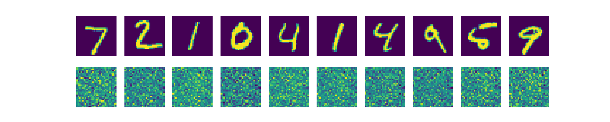
plt.savefig("sparse_autoencoder_result.png")

2. Run the script to sparse autoencoder.

python3 sparse_autoencoder.py

Training will run for 100 epochs and output a new image:

sparse_autoencoder_result.png

This image will show how the sparse model performs reconstruction using only a limited number of active neurons.

Step 5: Build a Deep Autoencoder

A Deep Autoencoder extends the architecture by stacking multiple encoding and decoding layers. This helps the model learn more abstract and hierarchical features from the data, making it more powerful than a shallow architecture.

1. Create a new script for a deep autoencoder.

nano deep_autoencoder.py

Add the following code.

import numpy as np
import matplotlib.pyplot as plt
import tensorflow as tf
from load_mnist import load_data

input_img = tf.keras.layers.Input(shape=(784,))
encoded = tf.keras.layers.Dense(128, activation='relu')(input_img)
encoded = tf.keras.layers.Dense(64, activation='relu')(encoded)
encoded = tf.keras.layers.Dense(32, activation='relu')(encoded)
decoded = tf.keras.layers.Dense(64, activation='relu')(encoded)
decoded = tf.keras.layers.Dense(128, activation='relu')(decoded)
decoded = tf.keras.layers.Dense(784, activation='sigmoid')(decoded)

autoencoder = tf.keras.models.Model(input_img, decoded)
autoencoder.compile(optimizer='adadelta', loss='binary_crossentropy')

(x_train, _), (x_test, _) = load_data()
x_train = x_train.astype('float32') / 255.
x_test = x_test.astype('float32') / 255.
x_train = x_train.reshape((len(x_train), 784))
x_test = x_test.reshape((len(x_test), 784))

autoencoder.fit(x_train, x_train, epochs=100, batch_size=256, shuffle=True, validation_data=(x_test, x_test))

decoded_imgs = autoencoder.predict(x_test)

# Visualize
n = 10
plt.figure(figsize=(20, 4))
for i in range(n):
    ax = plt.subplot(2, n, i + 1)
    plt.imshow(x_test[i].reshape(28, 28), cmap='gray')
    ax.axis('off')
    ax = plt.subplot(2, n, i + 1 + n)
    plt.imshow(decoded_imgs[i].reshape(28, 28), cmap='gray')
    ax.axis('off')
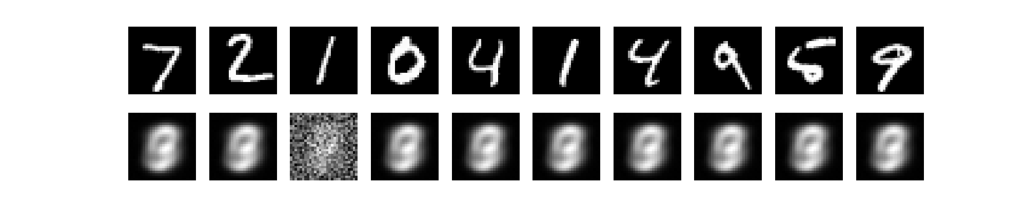
plt.savefig("deep_autoencoder_result.png")

2. Run the deep encoder.

python3 deep_autoencoder.py

Once complete, the output image deep_autoencoder_result.png will be saved in your working directory. It shows side-by-side comparisons of the original and reconstructed digits.

Step 6: Build a Convolutional Autoencoder

The Convolutional Autoencoder (CAE) is designed for image data. Instead of flattening the input, it uses convolutional layers to preserve spatial structure. This is ideal for capturing visual patterns in images like edges, curves, and textures. This model compresses the 28×28 grayscale image to a low-dimensional feature map, then reconstructs it.

1. Create a script for a convolutional autoencoder.

nano conv_autoencoder.py

Add the following code.

import numpy as np
import matplotlib.pyplot as plt
import tensorflow as tf
from load_mnist import load_data

(x_train, _), (x_test, _) = load_data()
x_train = x_train.astype('float32') / 255.
x_test = x_test.astype('float32') / 255.
x_train = np.reshape(x_train, (len(x_train), 28, 28, 1))
x_test = np.reshape(x_test, (len(x_test), 28, 28, 1))

input_img = tf.keras.layers.Input(shape=(28, 28, 1))
x = tf.keras.layers.Conv2D(16, (3, 3), activation='relu', padding='same')(input_img)
x = tf.keras.layers.MaxPooling2D((2, 2), padding='same')(x)
x = tf.keras.layers.Conv2D(8, (3, 3), activation='relu', padding='same')(x)
x = tf.keras.layers.MaxPooling2D((2, 2), padding='same')(x)
encoded = tf.keras.layers.Conv2D(8, (3, 3), activation='relu', padding='same')(x)

x = tf.keras.layers.UpSampling2D((2, 2))(encoded)
x = tf.keras.layers.Conv2D(8, (3, 3), activation='relu', padding='same')(x)
x = tf.keras.layers.UpSampling2D((2, 2))(x)
decoded = tf.keras.layers.Conv2D(1, (3, 3), activation='sigmoid', padding='same')(x)

autoencoder = tf.keras.models.Model(input_img, decoded)
autoencoder.compile(optimizer='adadelta', loss='binary_crossentropy')
autoencoder.fit(x_train, x_train, epochs=50, batch_size=128, shuffle=True, validation_data=(x_test, x_test))

decoded_imgs = autoencoder.predict(x_test)

n = 10
plt.figure(figsize=(20, 4))
for i in range(n):
    ax = plt.subplot(2, n, i + 1)
    plt.imshow(x_test[i].reshape(28, 28), cmap='gray')
    ax.axis('off')
    ax = plt.subplot(2, n, i + 1 + n)
    plt.imshow(decoded_imgs[i].reshape(28, 28), cmap='gray')
    ax.axis('off')
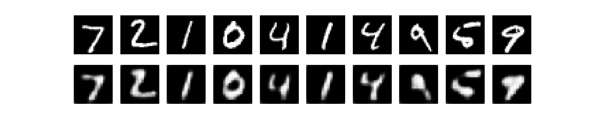
plt.savefig("conv_autoencoder_result.png")

2. Run the convolutional autoencoder.

python3 conv_autoencoder.py

After 50 epochs, the model will generate:

conv_autoencoder_result.png

This shows original and reconstructed digits using convolutional filters.

Step 7: Build a Denoising Autoencoder

The Denoising Autoencoder learns to reconstruct clean images from noisy input. It’s especially useful when working with real-world images that may be corrupted, blurred, or degraded.

In this section, we’ll artificially add Gaussian noise to the MNIST dataset and train the model to remove it.

1. Create a new Python script.

nano denoising_autoencoder.py

Add the following code.

import numpy as np
import matplotlib.pyplot as plt
import tensorflow as tf
from load_mnist import load_data

(x_train, _), (x_test, _) = load_data()
x_train = x_train.astype('float32') / 255.
x_test = x_test.astype('float32') / 255.
x_train = np.reshape(x_train, (len(x_train), 28, 28, 1))
x_test = np.reshape(x_test, (len(x_test), 28, 28, 1))

noise_factor = 0.5
x_train_noisy = np.clip(x_train + noise_factor * np.random.normal(size=x_train.shape), 0., 1.)
x_test_noisy = np.clip(x_test + noise_factor * np.random.normal(size=x_test.shape), 0., 1.)

input_img = tf.keras.layers.Input(shape=(28, 28, 1))
x = tf.keras.layers.Conv2D(32, (3, 3), activation='relu', padding='same')(input_img)
x = tf.keras.layers.MaxPooling2D((2, 2), padding='same')(x)
x = tf.keras.layers.Conv2D(32, (3, 3), activation='relu', padding='same')(x)
x = tf.keras.layers.MaxPooling2D((2, 2), padding='same')(x)
x = tf.keras.layers.Conv2D(32, (3, 3), activation='relu', padding='same')(x)
x = tf.keras.layers.UpSampling2D((2, 2))(x)
x = tf.keras.layers.Conv2D(32, (3, 3), activation='relu', padding='same')(x)
x = tf.keras.layers.UpSampling2D((2, 2))(x)
decoded = tf.keras.layers.Conv2D(1, (3, 3), activation='sigmoid', padding='same')(x)

autoencoder = tf.keras.models.Model(input_img, decoded)
autoencoder.compile(optimizer='adadelta', loss='binary_crossentropy')
autoencoder.fit(x_train_noisy, x_train, epochs=100, batch_size=128, shuffle=True, validation_data=(x_test_noisy, x_test))

decoded_imgs = autoencoder.predict(x_test_noisy)

n = 10
plt.figure(figsize=(20, 4))
for i in range(n):
    ax = plt.subplot(2, n, i + 1)
    plt.imshow(x_test_noisy[i].reshape(28, 28), cmap='gray')
    ax.axis('off')
    ax = plt.subplot(2, n, i + 1 + n)
    plt.imshow(decoded_imgs[i].reshape(28, 28), cmap='gray')
    ax.axis('off')
plt.savefig("denoising_autoencoder_result.png")

2. Run the denoising autoencoder.

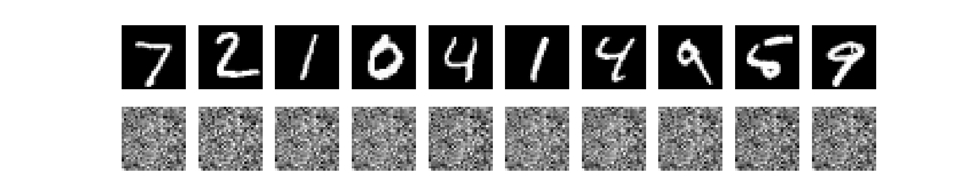
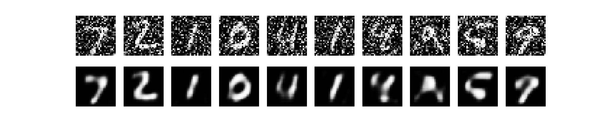
python3 denoising_autoencoder.py

After training completes, the result will be saved to.

denoising_autoencoder_result.png

This image will show the original noisy input on the top row and the clean, denoised output on the bottom.

Conclusion

In this tutorial, you built and tested five different types of autoencoders using Keras on an Ubuntu 24.04 GPU server. You started with a simple architecture, then explored sparse, deep, convolutional, and denoising autoencoders.

Each model helped you learn a new approach to image compression and reconstruction using neural networks. You also visualized the output of each model to compare how well it learned to recreate the MNIST digits.