How to Find Seasonality Patterns in Time Series Using Fourier Transforms on Ubuntu 24.04 GPU Server

Time series data often shows repeating cycles, called seasonality, such as weekly sales spikes or daily traffic peaks. Detecting these patterns is important for forecasting and decision-making.

The Fourier Transform is a powerful tool to uncover hidden cycles by breaking a signal into its frequency components. This makes it easy to spot dominant periodic trends like a 7-day weekly pattern.

In this tutorial, you’ll generate synthetic time series data, analyze it with NumPy (CPU), and then accelerate the process using CuPy (GPU) on Ubuntu 24.04.

Prerequisites

• An Ubuntu 24.04 server with an NVIDIA GPU.
• A non-root user or a user with sudo privileges.
• NVIDIA drivers are installed on your server.

Step 1 – Set Up a Python Environment

To keep your project organized and avoid conflicts with system-wide packages, it’s best to create a dedicated Python virtual environment.

1. First, install the required base tools.

apt install -y python3 python3-venv python3-pip git

2. Create an isolated environment.

python3 -m venv ts-env

3. Activate the environment.

source ts-env/bin/activate

4. Upgrade pip and install the libraries needed for time series analysis and GPU acceleration.

pip install --upgrade pip
pip install numpy matplotlib pandas
pip install cupy-cuda12x

Step 2 – Generate a Sample Time Series

To demonstrate how to detect seasonality, you’ll first create a synthetic dataset that mimics real-world time series data. This dataset will contain a weekly seasonal pattern combined with some random noise.

1. Open a new file called generate_timeseries.py.

nano generate_timeseries.py 

Add the following code.

#!/usr/bin/env python3
import numpy as np
import pandas as pd

# Generate a time index
days = pd.date_range(start="2024-01-01", periods=365, freq="D")

# Create seasonal pattern (weekly cycle) + noise
weekly_pattern = 10 * np.sin(2 * np.pi * np.arange(365) / 7)
noise = np.random.normal(0, 2, 365)
data = weekly_pattern + noise

# Save to CSV
df = pd.DataFrame({"date": days, "value": data})
df.to_csv("time_series.csv", index=False)

print("time_series.csv generated successfully")

2. Run the script.

python3 generate_timeseries.py 

A new file named time_series.csv will be created. It contains two columns: date and value, where value represents the seasonal signal plus noise.

time_series.csv generated successfully

Step 3 – Analyzing Seasonality with CPU-based FFT

Now that you have a synthetic dataset, the next step is to analyze it using the Fast Fourier Transform (FFT) with NumPy. This will let you uncover the hidden weekly cycle.

1. Create a new file called seasonality_fft.py.

nano seasonality_fft.py

Add the following code.

#!/usr/bin/env python3
import os
# Use a non-GUI backend if DISPLAY isn't set
if os.environ.get("DISPLAY", "") == "":
    import matplotlib
    matplotlib.use("Agg")

import pandas as pd
import numpy as np
import matplotlib.pyplot as plt

def main():
    df = pd.read_csv("time_series.csv", parse_dates=["date"])
    df = df.sort_values("date").reset_index(drop=True)

    # Estimate sampling interval (days) from timestamps
    deltas = df["date"].diff().dt.total_seconds().dropna() / 86400.0
    d = float(np.median(deltas)) if len(deltas) else 1.0  # default daily

    values = df["value"].to_numpy()
    n = len(values)

    fft_vals = np.fft.fft(values)
    fft_freq = np.fft.fftfreq(n, d=d)

    mask = fft_freq > 0
    positive_freqs = fft_freq[mask]
    positive_fft = np.abs(fft_vals[mask]) * (2.0 / n)  # scale amplitude

    plt.figure(figsize=(10, 5))
    plt.plot(positive_freqs, positive_fft, linewidth=1)
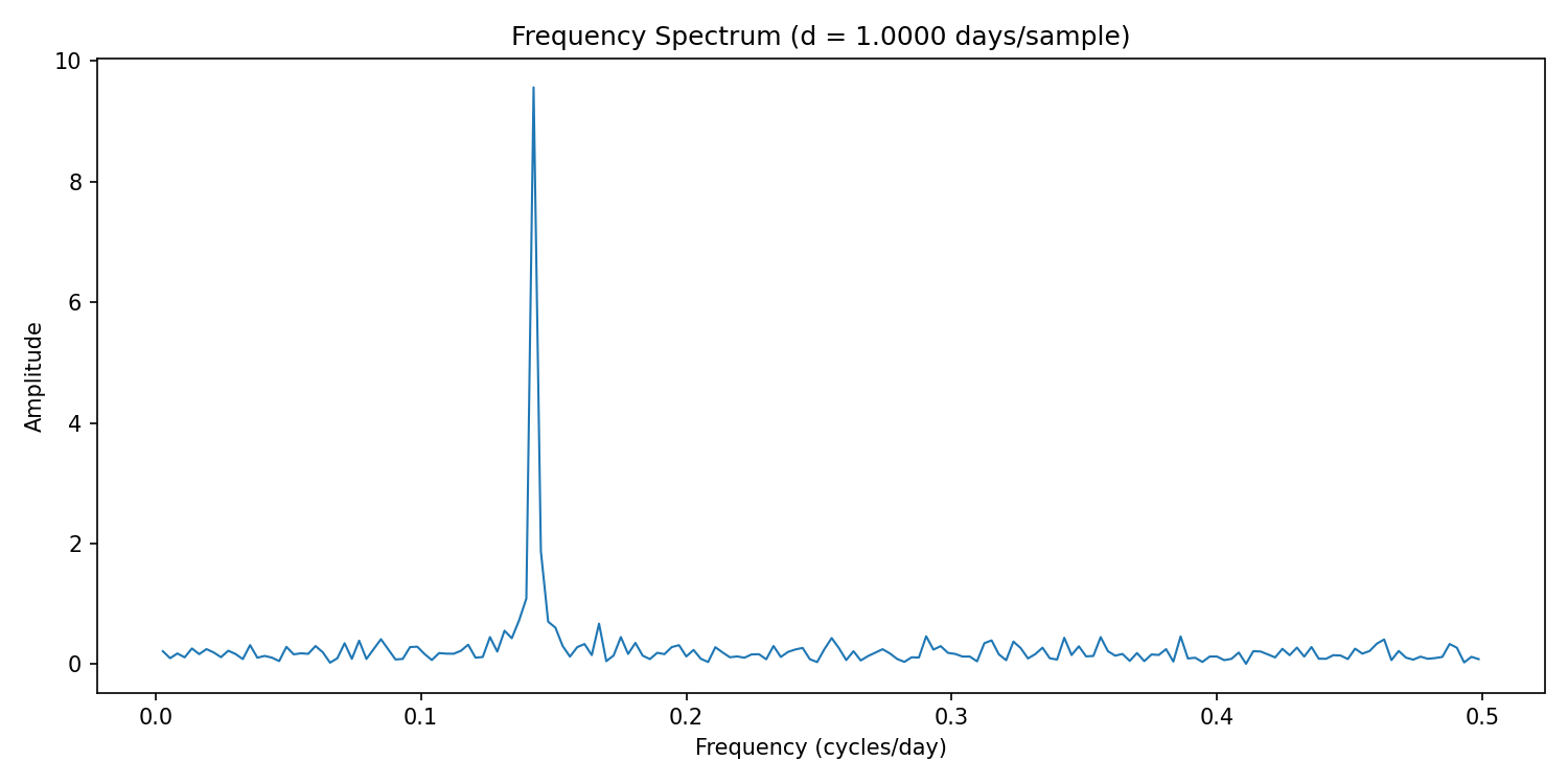
    plt.title(f"Frequency Spectrum (d = {d:.4f} days/sample)")
    plt.xlabel("Frequency (cycles/day)")
    plt.ylabel("Amplitude")
    plt.tight_layout()

    out = "fft_spectrum.png"
    plt.savefig(out, dpi=150)
    print(f"[OK] Saved spectrum to {out}")

    # Optional: print top 5 peaks
    top_idx = np.argsort(positive_fft)[-5:][::-1]
    print("\nTop 5 peaks:")
    for i in top_idx:
        freq = positive_freqs[i]
        period_days = 1.0 / freq if freq != 0 else float("inf")
        amp = positive_fft[i]
        print(f"  freq={freq:.6f} cycles/day  (~{period_days:.2f} days)  amplitude={amp:.4f}")

if __name__ == "__main__":
    main()

2. Run the script.

python3 seasonality_fft.py

You should see an output similar to:

[OK] Saved spectrum to fft_spectrum.png

Top 5 peaks:
  freq=0.142466 cycles/day  (~7.02 days)  amplitude=9.5641
  freq=0.145205 cycles/day  (~6.89 days)  amplitude=1.8724
  freq=0.139726 cycles/day  (~7.16 days)  amplitude=1.0879
  freq=0.136986 cycles/day  (~7.30 days)  amplitude=0.7250
  freq=0.147945 cycles/day  (~6.76 days)  amplitude=0.7032

The top peak at ~0.142 cycles/day corresponds to a 7-day cycle, which matches the weekly pattern you added earlier.

Step 4 – Accelerating FFT with GPU (CuPy)

While NumPy works well for small datasets, large-scale time series or real-time applications benefit from GPU acceleration. With CuPy, you can run the same FFT operations on the GPU, dramatically reducing computation time.

1. Create a new file called seasonality_fft_gpu.py.

nano seasonality_fft_gpu.py

Add the below code.

#!/usr/bin/env python3
import os
# Switch to non-GUI backend if no display
if os.environ.get("DISPLAY", "") == "":
    import matplotlib
    matplotlib.use("Agg")

import pandas as pd
import cupy as cp
import matplotlib.pyplot as plt

def main():
    # Load dataset
    df = pd.read_csv("time_series.csv", parse_dates=["date"])
    values = cp.array(df["value"].values)

    # FFT with GPU
    fft_vals = cp.fft.fft(values)
    fft_freq = cp.fft.fftfreq(len(values), d=1)

    # Convert back to NumPy for plotting
    mask = fft_freq > 0
    positive_freqs = cp.asnumpy(fft_freq[mask])
    positive_fft = cp.asnumpy(cp.abs(fft_vals[mask]))

    # Plot spectrum
    plt.figure(figsize=(10, 5))
    plt.plot(positive_freqs, positive_fft, linewidth=1)
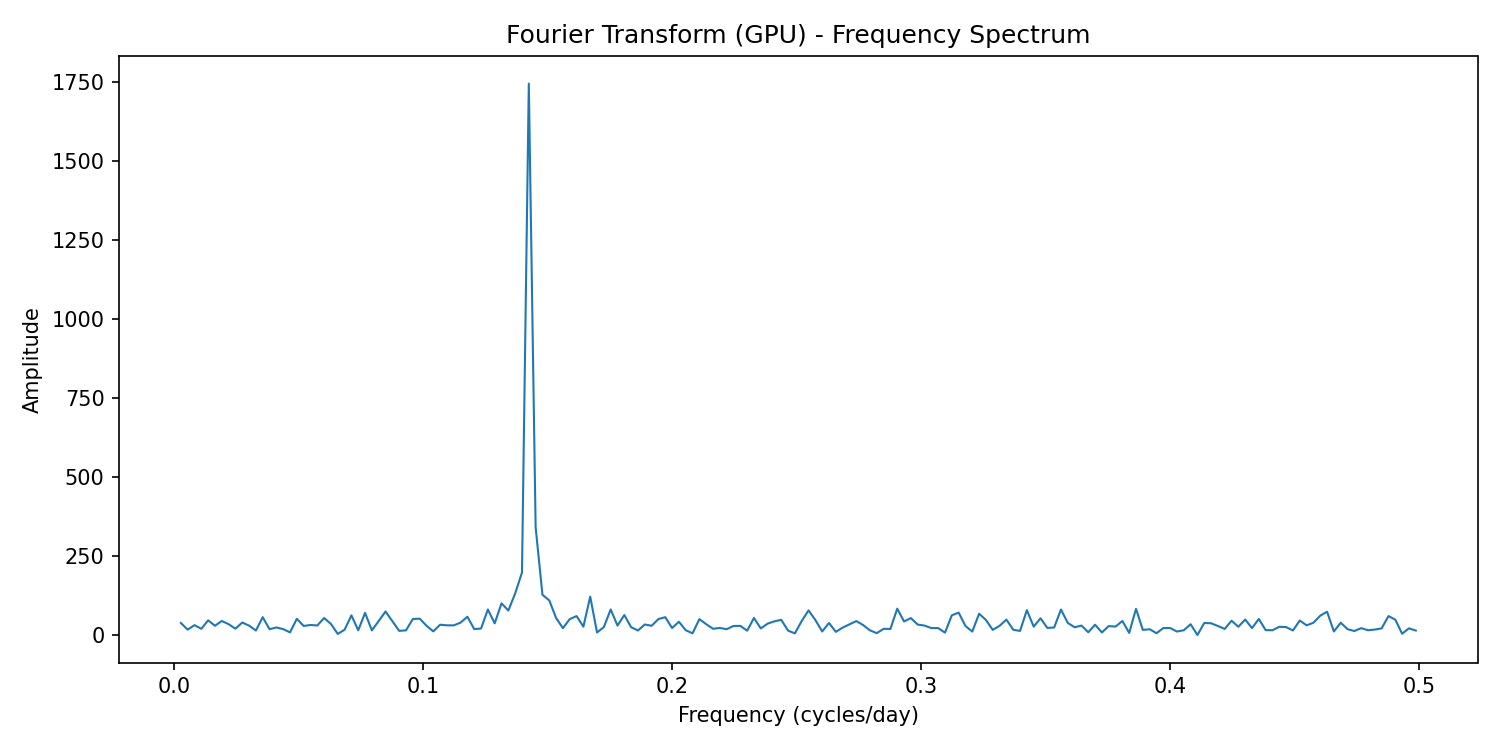
    plt.title("Fourier Transform (GPU) - Frequency Spectrum")
    plt.xlabel("Frequency (cycles/day)")
    plt.ylabel("Amplitude")
    plt.tight_layout()

    out_file = "fft_spectrum_gpu.png"
    plt.savefig(out_file, dpi=150)
    print(f"[OK] Spectrum saved to {out_file}")

    # Optional: show top 5 peaks
    import numpy as np
    top_idx = np.argsort(positive_fft)[-5:][::-1]
    print("\nTop 5 peaks:")
    for i in top_idx:
        freq = positive_freqs[i]
        period_days = 1.0 / freq if freq != 0 else float("inf")
        amp = positive_fft[i]
        print(f"  freq={freq:.6f} cycles/day  (~{period_days:.2f} days)  amplitude={amp:.4f}")

if __name__ == "__main__":
    main()

2. Run the script.

python3 seasonality_fft_gpu.py

Expected output:

[OK] Spectrum saved to fft_spectrum_gpu.png

Top 5 peaks:
  freq=0.142466 cycles/day  (~7.02 days)  amplitude=1745.4544
  freq=0.145205 cycles/day  (~6.89 days)  amplitude=341.7149
  freq=0.139726 cycles/day  (~7.16 days)  amplitude=198.5501
  freq=0.136986 cycles/day  (~7.30 days)  amplitude=132.3208
  freq=0.147945 cycles/day  (~6.76 days)  amplitude=128.3347

Here too, the dominant frequency (~0.142 cycles/day) corresponds to a 7-day weekly cycle. The difference is in amplitude scaling; GPU FFT outputs larger values, but the detected cycle remains the same.

Step 5 – Comparing CPU vs. GPU Results

At this point, you’ve analyzed the same dataset using both NumPy (CPU) and CuPy (GPU). Let’s look at how the results compare.

1. Frequency Detection

Both approaches identify the dominant peak around 0.142 cycles/day, which translates to roughly 7 days per cycle. This confirms that the weekly pattern we built into the synthetic dataset has been correctly detected.

2. Amplitude Differences

You may notice that the amplitude values from the GPU output are much larger than those from the CPU run. This difference comes from internal scaling in the libraries, but it doesn’t affect the interpretation of the frequency peaks. The relative size of peaks is what matters for identifying seasonality.

3. Performance

• CPU FFT (NumPy): Works well for small datasets like our 365-day series.

• GPU FFT (CuPy): Shines with large datasets, streaming data, or when you need to run FFT repeatedly in real time. On a GPU-enabled server, you’ll typically see much faster execution compared to CPU.

4. Visual Comparison

Both scripts save frequency spectrum plots (fft_spectrum.png for CPU and fft_spectrum_gpu.png for GPU). You’ll see the same dominant weekly cycle in both graphs, confirming that GPU acceleration doesn’t change the result, only the speed.

In short, CPU analysis is fine for small-scale work. Still, if you’re analyzing millions of points or running Fourier analysis as part of a production pipeline, GPU acceleration can make a big difference.

Conclusion

In this tutorial, you explored how to detect seasonality patterns in time series data using Fourier Transforms on an Ubuntu 24.04 GPU server. You began by setting up a clean Python environment with NumPy, Pandas, Matplotlib, and CuPy, then created a synthetic dataset containing a weekly cycle mixed with random noise. With this dataset, you applied a CPU-based FFT using NumPy to uncover the hidden seasonal component, and later accelerated the process with a GPU-based FFT using CuPy.