Predicting stock prices has long been a challenge for investors and analysts alike. With the advent of deep learning, particularly Long Short-Term Memory (LSTM) neural networks, we now have powerful tools to analyze time-series data like stock prices.
In this tutorial, we will walk through setting up an LSTM model on an Ubuntu 24.04 GPU server to predict stock prices, using Apple Inc. (AAPL) as an example.
Prerequisites
Before we begin, ensure you have:
- Ubuntu 24.04 server with GPU capabilities.
- Python 3 and NVIDIA drivers installed.
- Basic familiarity with terminal commands.
Step 1: Setting Up the Environment
First, let’s create a clean Python environment and install the necessary packages:
1. Install Python’s virtual environment and pip packages.
apt install python3-venv python3-pip2. Create a new virtual environment.
python3 -m venv stock_env3. Activate the environment.
source stock_env/bin/activate4. Install essential packages, including TensorFlow, for our LSTM model.
pip install tensorflow numpy pandas matplotlib scikit-learn yfinanceStep 2: Writing the LSTM Stock Prediction Script
Now, we will write the full Python script to download stock data, preprocess it, build and train the LSTM model, and visualize the predictions. This script handles everything: data download, training, evaluation, and next-day prediction.
Create the script file.
nano stock_prediction_lstm.pyAdd the following code.
import numpy as np
import pandas as pd
import yfinance as yf
import matplotlib.pyplot as plt
from sklearn.preprocessing import MinMaxScaler
from tensorflow.keras.models import Sequential
from tensorflow.keras.layers import LSTM, Dense, Dropout

# Download stock data directly
ticker = 'AAPL'
data = yf.download(ticker, start='2010-01-01', end='2025-04-20')

# Preprocess data
data_close = data[['Close']]
dataset = data_close.values

# Scale data between 0 and 1
scaler = MinMaxScaler(feature_range=(0, 1))
scaled_data = scaler.fit_transform(dataset)

# Split into training (80%) and testing (20%)
train_len = int(len(scaled_data) * 0.8)
train_data = scaled_data[:train_len]

# Function to create dataset for LSTM
def create_dataset(data, time_step=60):
    X, y = [], []
    for i in range(time_step, len(data)):
        X.append(data[i-time_step:i, 0])
        y.append(data[i, 0])
    return np.array(X), np.array(y)

# Prepare training data
X_train, y_train = create_dataset(train_data)
X_train = X_train.reshape(X_train.shape[0], X_train.shape[1], 1)

# Build the LSTM model
model = Sequential([
    LSTM(50, return_sequences=True, input_shape=(X_train.shape[1], 1)),
    Dropout(0.2),
    LSTM(50, return_sequences=False),
    Dropout(0.2),
    Dense(25),
    Dense(1)
])

model.compile(optimizer='adam', loss='mean_squared_error')

# Train the model
model.fit(X_train, y_train, batch_size=32, epochs=50)
model.save('lstm_stock_model.h5')

# Prepare test data
test_data = scaled_data[train_len - 60:]
X_test, y_test = create_dataset(test_data)
X_test = X_test.reshape(X_test.shape[0], X_test.shape[1], 1)

# Predict and inverse transform
predictions = model.predict(X_test)
predictions = scaler.inverse_transform(predictions)
y_test_actual = scaler.inverse_transform(y_test.reshape(-1, 1))

# Calculate RMSE
rmse = np.sqrt(np.mean((predictions - y_test_actual)**2))
print(f"Root Mean Squared Error (RMSE): {rmse}")

# Visualization
train = data_close[:train_len]
valid = data_close[train_len:].copy()
valid['Predictions'] = predictions

plt.figure(figsize=(16, 8))
plt.title('Stock Price Prediction with LSTM')
plt.xlabel('Date')
plt.ylabel('Close Price (USD)')
plt.plot(train['Close'], label='Train')
plt.plot(valid['Close'], label='Actual')
plt.plot(valid['Predictions'], label='Predicted')
plt.legend()
plt.savefig('stock_prediction_plot.png')
plt.show()

# Predict the next day's closing price
def predict_next_day(model, data, scaler, time_step=60):
    last_60_days = data[-time_step:].values
    last_60_scaled = scaler.transform(last_60_days)
    X_pred = np.array([last_60_scaled])
    X_pred = X_pred.reshape(X_pred.shape[0], X_pred.shape[1], 1)
    pred_price = model.predict(X_pred)
    return scaler.inverse_transform(pred_price)[0][0]

next_day_price = predict_next_day(model, data_close, scaler)
print(f"Predicted next day price for {ticker}: ${next_day_price:.2f}")
The above code:
- Downloads historical stock data for AAPL from Yahoo Finance.
- Trains an LSTM neural network to predict the future closing price based on past data.
- Visualizes the model’s predicted vs. actual closing prices.
- Predicts and displays the next day’s closing price for Apple’s stock.
Step 3: Run the Model
Now let’s run the script to train the model and see the results.
python3 stock_prediction_lstm.pyThis step executes the prediction workflow and shows model accuracy and forecast.
Root Mean Squared Error (RMSE): 7.07722469189058
1/1 ━━━━━━━━━━━━━━━━━━━━ 0s 25ms/step
Predicted next day price for AAPL: $182.96
Step 4: Download the Prediction Chart
To visualize the chart on your local system, use scp to download it.
scp root@YOUR_SERVER_IP:/root/stock_prediction_plot.png Downloads/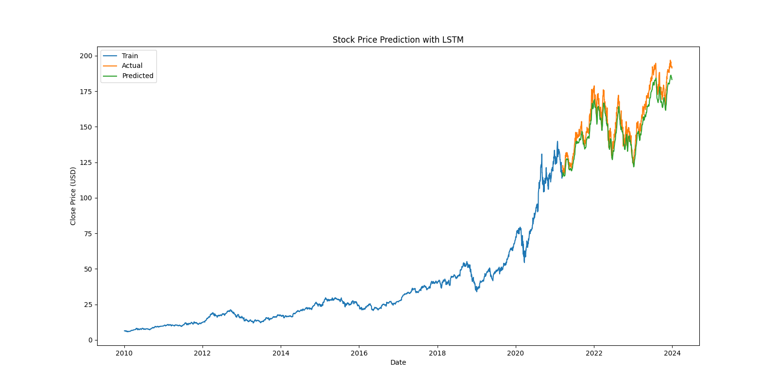
Conclusion
In this guide, you learned how to predict stock prices using an LSTM neural network on an Ubuntu 24.04 GPU server. We used Python and deep learning tools to download historical stock data, train a model, and predict the next day’s closing price for Apple’s stock. We also visualized the model’s performance and saved the results for easy access.
* This post is for informational purposes only and does not constitute professional, legal, financial, or technical advice. Each situation is unique and may require guidance from a qualified professional.
Readers should conduct their own due diligence before making any decisions.