Implementing Autoencoders from Scratch in PyTorch on Ubuntu 24.04 GPU Server

Autoencoders are a special type of neural network used to learn efficient representations of data, often for the purpose of dimensionality reduction or unsupervised feature learning. They work by compressing the input into a latent space (encoding) and then reconstructing the original input from this compressed version (decoding). The main goal is to output data that closely resembles the input.

In this tutorial, you’ll learn how to implement an autoencoder from scratch in PyTorch, without using high-level prebuilt models. You’ll train it on the MNIST dataset, which contains handwritten digits, and use a fully connected (linear) architecture to build both the encoder and decoder.

Prerequisites

• An Ubuntu 24.04 server with an NVIDIA GPU.
• A non-root user or a user with sudo privileges.
• NVIDIA drivers are installed on your server.

Step 1: Set up Python Environment

Before diving into the code, you’ll need to set up a clean Python development environment on your Ubuntu 24.04 GPU server. Follow these steps to install the necessary packages and verify CUDA support.

1. Install system dependencies for managing your project.

apt install python3 python3-pip python3-venv build-essential git -y

2. Create and activate a Python virtual environment.

python3 -m venv autoencoder
source autoencoder/bin/activate

3. Upgrade pip and install required Python packages.

pip install --upgrade pip
pip install matplotlib
pip install torch torchvision torchaudio --index-url https://download.pytorch.org/whl/cu121

4. Check if your GPU is detected by PyTorch.

python3 -c "import torch; print(torch.cuda.is_available())"

Output.

True

5. Create a project directory.

mkdir pytorch_autoencoder
cd pytorch_autoencoder

You’ll place all your scripts (dataset loader, model, training loop, and visualization) inside this directory.

Step 2: Prepare the Dataset Loader

To train our autoencoder, we’ll use the MNIST dataset, a classic benchmark in machine learning containing 28×28 grayscale images of handwritten digits (0–9). PyTorch’s torchvision.datasets module makes it easy to download and use this dataset.

Create a Python script to wrap the dataset and data loader logic.

nano dataset.py

Add the following code.

# dataset.py
import torch
from torchvision import datasets, transforms
from torch.utils.data import DataLoader

def get_dataloaders(batch_size=128):
    transform = transforms.ToTensor()

    train_dataset = datasets.MNIST(root='data', train=True, transform=transform, download=True)
    test_dataset = datasets.MNIST(root='data', train=False, transform=transform, download=True)

    train_loader = DataLoader(train_dataset, batch_size=batch_size, shuffle=True)
    test_loader = DataLoader(test_dataset, batch_size=batch_size, shuffle=False)

    return train_loader, test_loader

Explanation:

• transforms.ToTensor(): Converts images to tensors and scales pixel values from [0, 255] to [0, 1].
• datasets.MNIST(…): Automatically downloads the MNIST dataset.
• DataLoader(…): Creates iterable batches for training and testing.

Step 3: Build the Autoencoder Model

Now that the dataset loader is ready, it’s time to build the core of this project, the Autoencoder model. We’ll define a simple feedforward neural network with two main parts:

Encoder: Compresses the input image into a lower-dimensional representation.
Decoder: Reconstructs the image from this compressed version.

Create a autoencoder.py file.

nano autoencoder.py

Add the following code.

# autoencoder.py
import torch.nn as nn

class Autoencoder(nn.Module):
    def __init__(self):
        super(Autoencoder, self).__init__()
        self.encoder = nn.Sequential(
            nn.Linear(28 * 28, 128),
            nn.ReLU(),
            nn.Linear(128, 64),
            nn.ReLU()
        )
        self.decoder = nn.Sequential(
            nn.Linear(64, 128),
            nn.ReLU(),
            nn.Linear(128, 28 * 28),
            nn.Sigmoid()
        )

    def forward(self, x):
        x = x.view(x.size(0), -1)
        encoded = self.encoder(x)
        decoded = self.decoder(encoded)
        return decoded

Explanation of the Model

• Input: MNIST images are 28×28, so we flatten them to a 784-element vector.
• Encoder: 784 → 128 → 64: Two linear layers with ReLU activation.
• Decoder: 64 → 128 → 784: Two linear layers that attempt to reconstruct the original image.
• Final activation (Sigmoid): Scales outputs between 0 and 1 (same range as input pixels).

Step 4: Train the Autoencoder

With the dataset and model in place, it’s time to train the autoencoder.

Let’s create a Python file.

nano train.py

Add the following code.

# train.py
import torch
import torch.nn as nn
import torch.optim as optim
from autoencoder import Autoencoder
from dataset import get_dataloaders

device = torch.device("cuda" if torch.cuda.is_available() else "cpu")

# Load data
train_loader, _ = get_dataloaders()

# Initialize model
model = Autoencoder().to(device)
criterion = nn.MSELoss()
optimizer = optim.Adam(model.parameters(), lr=1e-3)

# Training
num_epochs = 10
for epoch in range(num_epochs):
    total_loss = 0
    for imgs, _ in train_loader:
        imgs = imgs.to(device)
        outputs = model(imgs)
        loss = criterion(outputs, imgs.view(imgs.size(0), -1))

        optimizer.zero_grad()
        loss.backward()
        optimizer.step()

        total_loss += loss.item()

    print(f"Epoch [{epoch+1}/{num_epochs}], Loss: {total_loss / len(train_loader):.4f}")

# Save the model
torch.save(model.state_dict(), "autoencoder.pth")

Execute the training script to start training your autoencoder.

python3 train.py

A trained model file autoencoder.pth will be saved in your working directory.

Step 5: Visualize the Output

In this step, you’ll load your saved model (autoencoder.pth), pass test images through the autoencoder, compare original and reconstructed images, save the output as a visual .png file.

Create visualize.py file.

nano visualize.py

Add the following code.

# visualize.py
import torch
from autoencoder import Autoencoder
from dataset import get_dataloaders
import matplotlib.pyplot as plt

device = torch.device("cuda" if torch.cuda.is_available() else "cpu")

# Load model
model = Autoencoder().to(device)
model.load_state_dict(torch.load("autoencoder.pth"))
model.eval()

# Get test images
_, test_loader = get_dataloaders()
images, _ = next(iter(test_loader))
images = images[:8].to(device)

# Reconstruct
with torch.no_grad():
    reconstructed = model(images)

images = images.cpu()
reconstructed = reconstructed.view(-1, 1, 28, 28).cpu()

# Plot
fig, axs = plt.subplots(2, 8, figsize=(12, 3))
for i in range(8):
    axs[0, i].imshow(images[i].squeeze(), cmap='gray')
    axs[1, i].imshow(reconstructed[i].squeeze(), cmap='gray')
    axs[0, i].axis("off")
    axs[1, i].axis("off")
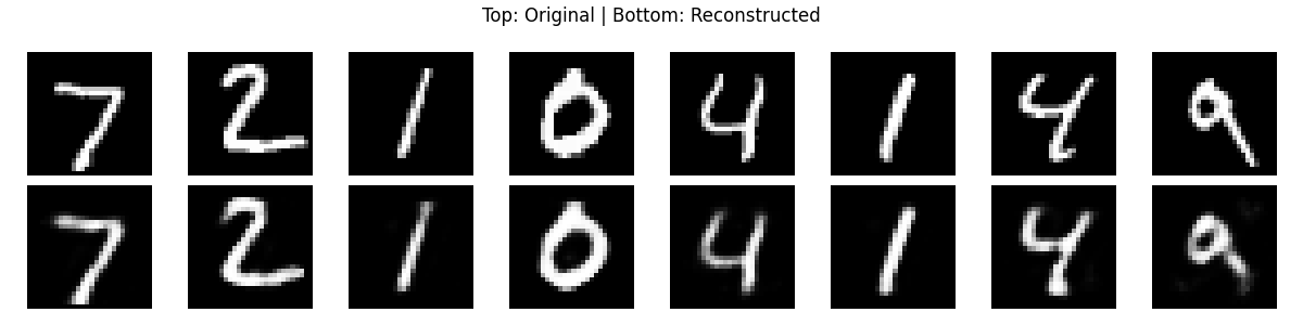
plt.suptitle("Top: Original | Bottom: Reconstructed")
plt.tight_layout()
plt.savefig("reconstructed.png")
plt.show()

Run the visualization script.

python3 visualize.py

This will generate a file reconstructed.png showing original and reconstructed digits side by side.

Step 6: Download the Result to Your Local Machine

From your local desktop computer, run this scp command to copy the image from your server.

scp root@your-server-ip:/root/pytorch_autoencoder/reconstructed.png /home/user/Downloads/

Open the downloaded image file to view the reconstructed.png file.

Conclusion

In this tutorial, you learned how to implement an autoencoder from scratch in PyTorch on an Ubuntu 24.04 GPU server. You set up a clean Python environment, built a custom encoder–decoder architecture using fully connected layers, trained it on the MNIST dataset, and visualized how well the model could reconstruct digit images.